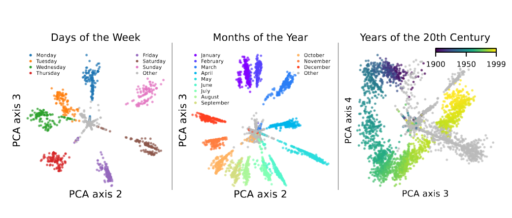
Figure 1:Features corresponding to the days of the week, months of the year, and years of the 20th century in layer 7 of GPT2-small appear to lie on a circle. The representations are obtained using an SAE and examining reconstructions after ablating all other SAE features, e.g. the points for days of the week are obtained by examining the representation of weekdays after passing through an SAE where all features are set to 0 except for the feature corresponding to weekdays (and a cluster that are closely related). Taken from Engels et al. (2024).
Recent work Engels et al. (2024), Modell et al. (2025) showed that language models represent some features as multi-dimensional manifolds in activation space. A prime example (Figure 1) is “days of the week” forming a circle. My previous post explains multidimensional features and the SAE-based discovery method. In brief: train an SAE on an MLP layer, cluster columns of the decoder matrix by cosine similarity, then for each cluster: (1) collect tokens strongly activating cluster features, (2) pass their activations through the SAE with non-cluster features ablated, yielding a point cloud in , (3) manually inspect low-dimensional PCA projections for geometric structure.
This approach has two key limitations:
Manual inspection doesn’t scale
Low-dimensional PCA projections may miss nontrivial geometry in high-dimensional spaces (e.g. for GPT-2) Both works note that they find surprisingly few multidimensional features, perhaps this is attributable to the two reasons above among others.
In a previous life, I worked on topological deep learning, more precisely using invariants from algebraic topology as components in ML loss functions. The following work is an attempt to use these topological invariants to address the limitations above.
1Background on Persistent Homology
Over the past two decades, topological data analysis (TDA) has emerged as a powerful new tool that leverages tools from algebraic topology to study the underlying “shape of data”.
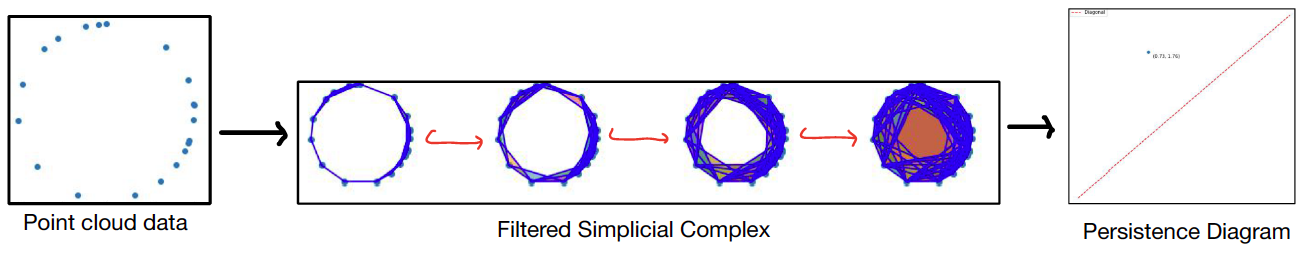
Figure 2:The single parameter persistence pipeline.
Classical or single parameter persistent homology was developed in the early 2000s by Carlsson, Edelsbrunner, and Harer as an extension of simplicial homology to discrete data sets. It accomplishes this by constructing a filtered simplicial complex and tracking the evolution of simplicial homology across the filtration. This information is encoded in a persistence module, which can be characterized up to isomorphism by a persistence barcode or diagram. We point the reader to Carlsson & Vejdemo-Johansson (2021) for a comprehensive survey.
A short overview adapted from my master’s thesis is provided below.
TL;DR - given a point cloud we can compute the -th persistence diagram. Points far away from the diagonal indicate significant -dimensional “circles” in the point cloud. In the one-dimensional case, for example, we detect circles (ideally the reconstruction plot of the days of the week Figure 1 would show a circle in its persistence diagram).
1.1Filtrations and homology
Persistent homology uses simplicial homology to study geometric features of point cloud data by producing a persistence diagram (or barcode) for a given point cloud . We introduce this pipeline using an example. For a more comprehensive introduction, see Carlsson (2009), Edelsbrunner & Morozov (2013) or Oudot (2015).
The prototypical example used to demonstrate the persistent homology pipeline is the dataset depicted in Figure 3.
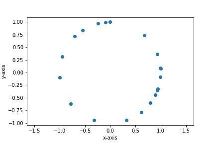
Figure 3:Data set consisting of 20 points sampled from the unit circle.
Visually, we see immediately that appears to be sampled from a circle. Algebraic topology and in particular simplicial homology Hatcher (2002) is the perfect tool to formalize this intuition: 0-dimensional homology detects connected components, 1-dimensional homology detects circles, 2-dimensional homology detects spheres, and so on. It is easy to compute, especially over , and has many desirable properties such as functoriality and homotopy invariance.
Unfortunately, simply interpreting as a set of 0-simplices and applying simplicial homology delivers the following underwhelming result:
Ideally, we would like to see a single connected component being captured by 0-dimensional homology and non-trivial 1-dimensional homology to reflect the circular geometry of .
Instead of naively applying simplicial homology to a point cloud , we first construct a filtered simplicial complex using the points of . The idea here is to track the evolution of topological features as we change a certain parameter. We can then discern important topological features of the data from those arising from noise by looking at which features persist through the filtration. In the 1-parameter case, one works with filtrations indexed over the posets , or .
There are multiple ways to construct a filtered simplicial complex from point cloud data, but the most common one is the Vietoris-Rips (VR) complex.
Intuitively, one begins with the points as vertices. An edge connecting two points is then added to if and only if the two points are within a distance ; the triangle spanning points , and is included if and only if all the points lie within of each other, and so on. The Vietoris-Rips complex of the dataset from Figure 3 is illustrated in Figure 4. Note that since we are solely interested in 1-dimensional persistent homology, only the 1- and 2-simplices are displayed. The primary one dimensional topological feature (the circle) of the data persists through a significant portion of the filtration.
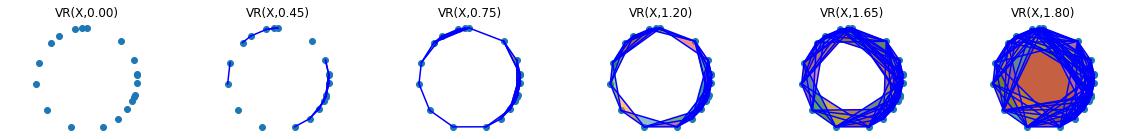
Figure 4:The 0-, 1-, and 2-simplices of the VR complex of a noisy circle.
1.2Persistence Modules
To track the evolution of topological features across a filtration, we compute -dimensional homology (over an arbitrary but fixed field ) for each subcomplex in the filtration. In the 1-parameter case, where , we obtain a sequence of vector spaces
where the maps are induced by the inclusion maps of the subcomplexes in the filtration (for the mathematically inclined this works because simplicial homology is a functor). This is an example of a persistence module. Thus the -dimensional persistence module of a filtration tracks how -dimensional cycles evolve over the filtration.
Applying 1-dimensional homology over to the filtration in Figure 4, we obtain
This is a special kind of persistence module known as an interval module, since it is an indicator module supported on an interval. It turns out that one can decompose persistence modules into a sum of interval modules.
1.3Persistence Barcodes and Diagrams
The barcode provides two equivalent visual summaries that are used in practice to interpret the topological features of the data. The barcode is obtained by simply plotting the intervals obtained from the decomposition. In this case, each bar corresponds to the lifespan of a cycle and hence longer bars represent features that characterize the geometry of the data while shorter bars may be attributed to noise.
Alternatively, given an interval in the barcode, one can plot the point . Doing this for each interval in the barcode results in the persistence diagram. Note that all points in the persistence diagram must lie above the diagonal, since a feature must have a nonnegative lifespan. Points far above the diagonal represent persistent features, while those lying near the diagonal are short-lived features attributable to noise. The 1-dimensional persistence barcode and diagram of the noisy circle is depicted in Figure 5 and as desired the circular nature of the dataset has been isolated.
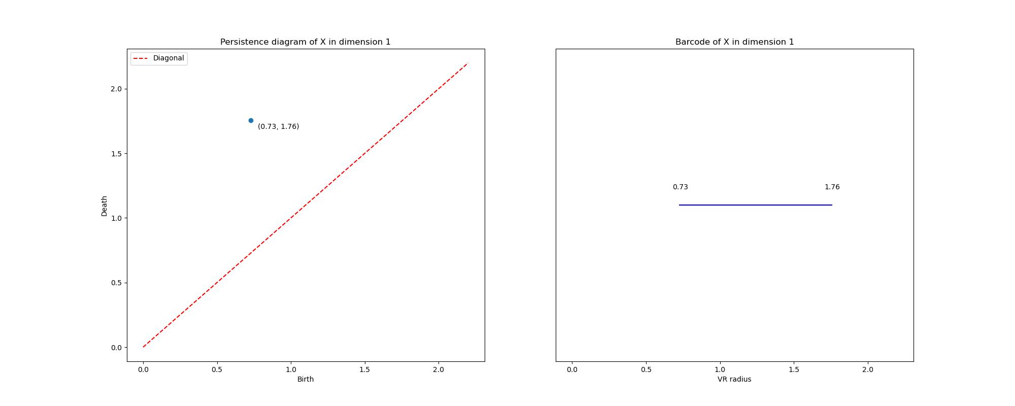
Figure 5:The 1-dimensional persistence diagram and barcode of the noisy circle from Figure 3 (computed using Gudhi Editorial Board (n.d.)).
We call the map that associates to a filtration of a finite simplicial complex its persistence diagram or barcode, the persistence map and denote it by . This map has many nice properties including that it is stable and differentiable almost everywhere.
2Using Persistent Homology to Find Multidimensional Feature Manifolds
Can we use persistent homology to automate the search for feature manifolds and address the limitations of the manual inspection approach? The following approach is inspired by Maggs et al. (2025), where the authors aim to detect circular structure in single-cell RNAseq data. The setting is strikingly similar: gene expression data is extremely high dimensional (on the order of 104) and for various biological reasons, detecting cyclic patterns in gene expression is of interest. Recall the setting we left off with in the previous post. We are given:
A language model and an MLP layer of interest. Given a token , the MLP layer produces an activation vector in .
A sparse autoencoder (SAE) with latent dimension . Note that the decoder matrix has dimension and we wish to find examples of multidimensional representations such as Figure 1.
Column of the decoder matrix of an SAE can be thought of as the projection of the basis vector of down to the lower dimensional space.
The first step in doing so is the same as Engels et al. (2024), i.e. we cluster the dictionary elements (columns of the decoder matrix of the SAE) using either spectral or graph methods into clusters where the dictionary elements have high cosine similarity (indicating that they represent similar concepts). We refer to Appendix F of Engels et al. (2024) for details on clustering, but for our purposes we can assume that we have clusters of feature directions. The question now boils down to: given a cluster of feature directions, do the model’s representations form a multidimensional manifold?
There’s a lot of notation in Definition 4, but all we’re doing is collecting tokens that activate the features in the cluster of interest () and then computing the reconstructions of these tokens using only the features in the cluster (in other words, ablating all feature directions except those in the cluster of interest). The reconstruction point cloud lives in and the projection of the reconstruction point cloud for the days of the week cluster is precisely what is depicted in Figure 1.
2.1Ring scores
Given a reconstruction point cloud, we can use persistent homology to assign it a ring score, i.e. a measure of the point cloud having a pronounced “hole”. Although we do not need to project down to the first three PCA components as in the manual inspection case, we still need to project down to a lower dimensional subspace, in the original space points are very unlikely to form any interesting geometric structure because of how “empty” such a high dimensional space is. We propose to examine the first 20 PCA components. The following definitions are taken directly from Maggs et al. (2025), the key idea here is that ring scores provide a neat summary statistic for a point cloud that captures how “circular” a point cloud is. It takes into account scaling by normalizing by the diameter of the point cloud, we should not be able to inflate scores by simply pushing points further apart. In the following we focus on 1-dimensional persistence, i.e. capturing circular features, though in principle the same pipeline can be used for higher dimensional analogs. Denote by
the persistence diagram of the projection of the reconstruction point cloud, where the birth-death pairs are sorted such that their corresponding persistence life spans, , are in decreasing order, i.e. .
The idea is that higher ring scores indicate a dominant circular feature, with capturing the lifespan of this feature and the other points in the persistence diagram representing features that obscure this prominent feature. Next, we need to choose a normalization factor to account for scaling, i.e. given a point cloud and a scaled version of the same point cloud , the ring score should be invariant. In Euclidean space, choosing accounts for this scaling; we refer to Maggs et al. (2025) for details. Finally, there has been a growing interest in studying persistence ratios , as opposed to persistence life spans, . We note that when using persistence ratios as opposed to life spans, there is no shape with a maximal -to-diameter ratio and so in this case we simply set the normalization factor to be . Thus we define the following two families of ring scores:
2.1.1Ring score significance
We can compute both diameter and ratio ring scores for each cluster of dictionary elements using the procedure above. This yields a null distribution of both ring scores, which we can then use to estimate a nominal -value for both the diameter and ratio ring scores of a given cluster. This allows us to immediately isolate candidate multidimensional features that have prominent cycles.
3Theoretical limitations
There are numerous issues with the current implementation that are addressed in the next section, that I believe can be solved by a mix of increased compute and some improvements to the way certain things are computed. However, there are also significant theoretical limitations to this approach that I want to address here. The most significant of these is that persistence-based methods detect cyclic structure, and if features had multi-dimensional but not cyclic structure these would likely be missed by this approach. Still, at least theoretically, the features presented in Engels et al. (2024), Modell et al. (2025) should be captured by persistence-based techniques.
Another limitation is not inherent to using persistence but rather to ring scores (at least in the way they are defined above) as a summary statistic. These ring scores were designed with detection of a single prominent cycle in mind. While this makes sense in the genomics context, in the feature manifold setting we would also be interested in feature manifolds with multiple prominent cycles, in fact these might be even more interesting than a single cycle feature. One theoretical extension might be to adapt the ring scores to address this.
4Operationalization and results
As hinted at above, the results from using the pipeline above were less than stellar, though I think this has more to do with the way I computed , e.g. I only sampled 1M tokens from the Pile or the fact that I used a pre-trained SAE Bloom et al. (2024) whereas Engels et al. (2024) train their own SAEs to suit this task. One fact that points to this is that I was not able to recover Figure 1 in any of my reconstructions. Another possible improvement to mitigate this is to look for tokens that activate with high frequency on a certain SAE feature and with a high score as in Templeton et al. (2024). This might lead to cleaner results with the tokens in a given being more clearly related to each other which is not the case in the current implementation. In fact, in order to even isolate clusters that might plausibly be related to temporal concepts like days of the week (in an attempt to reproduce Engels et al. (2024)), I had to search through the contexts of the top activating tokens as well.
The code can be found at this GitHub repo.
4.1Implementation details
Coming from a math background, this was one of my first projects working with a relatively large dataset and attempting to architect a large codebase (as opposed to my earlier mathematical code which was primarily single scripts or Jupyter notebooks). I learned a lot in the process including how to deploy code to a Kubernetes cluster, monitor using Weights and Biases, and I definitely still have a lot to learn when it comes to software engineering!
I made some unconventional choices in this project, one of which was to adapt and build on the excellent codebase that accompanies Simon & Zou (2025). This is code that uses SAEs to analyze protein language models that I came across while working on a different project (stay tuned!) and my code adapts it for use with LLMs. This is a very weird thing to do, because the PLM code was likely written because there’s no equivalent to TransformerLens Nanda & Bloom (2022) and Bloom et al. (2024) for PLMs and so this had to be built from the ground up. I could’ve (and arguably should’ve) used Nanda & Bloom (2022) out of the box, but I’m new to mech interp and I wanted to get my hands dirty. The PLM codebase is extremely well-written and (with the help of Claude and a holiday weekend) digging through InterPLM helped me understand the software engineering aspect of mech interp much better. Re-engineering it for LLMs was a very nice exercise. It was also my first time using Claude Code extensively and I found it to be incredibly useful when used right. In particular, I used it primarily to generate docstrings, tests, rename and refactor for readability. I also found it to be extremely helpful in generating Dockerfiles and job scripts. Finally, as I scaled to use more tokens, I found my code to be rather slow and while I knew that there was ample room for parallelization and knew which pieces of code could be parallelized, I wasn’t sure how precisely to do this. Instructing Claude to parallelize small chunks of code with precise instructions on how to parallelize worked very well and I did in fact learn some new tricks. Overall, I do not think that I could’ve coded this up over the Christmas break without LLM aid. That being said, this code has a lot of room for improvement and as mentioned above, I think these improvements will deliver the expected results while in its current state the results are underwhelming.
Specs:
LLM: GPT2-Small
Layer: 6
SAE: gpt2-small-res-jb - Pretrained from Bloom et al. (2024) with dictionary size 24576
Token dataset: Pile uncopyrighted
Number of tokens sampled to compute top tokens per SAE feature direction: 1 million Other configuration parameters available in the README.
4.2Results
4.2.1Spectral clustering
Below are the results when we cluster using spectral methods with n_clusters = 1000 and k=2.
Table 1:Significant (Spectral) Clusters (p < 0.05). Table depicts the 5 clusters with highest diameter and ratio scores respectively as well as the clusters containing temporal concepts (whose p-values are under 0.05) such as days of the week, months of the year, seasons, or times in the top activating tokens (or their context). Significance: * p<0.05, ** p<0.01
| Cluster | Type | Diam. Score | Diam. p-val | Ratio Score | Ratio p-val | ||
|---|---|---|---|---|---|---|---|
| 15 | Top 5 Diam | 0.0648 | 0.0050 | ** | 1.2309 | 0.3035 | |
| 111 | Top 5 Diam | 0.0558 | 0.0050 | ** | 1.2861 | 0.1791 | |
| 514 | Top 5 Diam | 0.0556 | 0.0050 | ** | 1.3927 | 0.0498 | * |
| 426 | Top 5 Diam | 0.0551 | 0.0050 | ** | 1.4290 | 0.0448 | * |
| 658 | Top 5 Diam | 0.0550 | 0.0050 | ** | 1.3416 | 0.0597 | |
| 165 | Temporal | 0.0281 | 0.0249 | * | 1.3251 | 0.0796 | |
| 634 | Top 5 Ratio | 0.0145 | 0.1642 | 1.5748 | 0.0100 | ** | |
| 891 | Top 5 Ratio | 0.0074 | 0.3035 | 1.8202 | 0.0050 | ** | |
| 682 | Top 5 Ratio | 0.0053 | 0.3184 | 1.6941 | 0.0050 | ** | |
| 878 | Temporal | 0.0029 | 0.3284 | 1.3822 | 0.0498 | * | |
| 335 | Top 5 Ratio | 0.0023 | 0.3582 | 1.7388 | 0.0050 | ** | |
| 436 | Temporal | 0.0018 | 0.3980 | 1.3735 | 0.0498 | * | |
| 848 | Temporal | 0.0019 | 0.3980 | 1.4371 | 0.0448 | * | |
| 719 | Temporal | 0.0014 | 0.5025 | 1.5060 | 0.0100 | ** | |
| 835 | Top 5 Ratio | 0.0013 | 0.5274 | 1.5386 | 0.0100 | ** |
Although the -values look promising, delving into the reconstruction plots and the tokens that activate them is less so. Consider for example cluster 426 which has significant nominal -values for both the diameter and ratio scores.
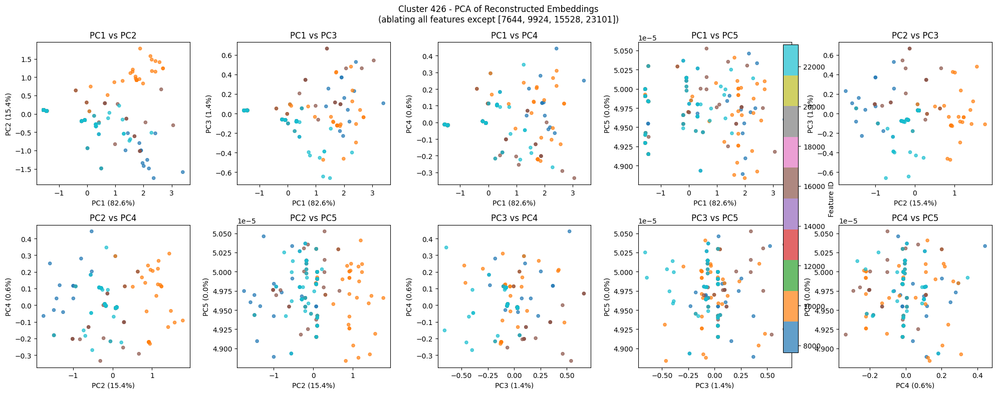
Figure 6:A few PCA components of the reconstruction point cloud for cluster 426. Note that the persistence diagram below is not computed on just the 2-dimensional projection.
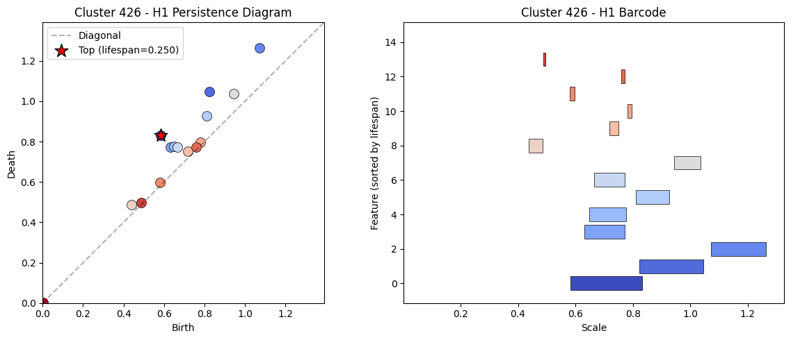
Figure 7:Persistence diagram (and equivalently barcode) for cluster 426.
We can see evidence of multiple small cycles in a few of the PCA components in Figure 6 and this corresponds to the three larger bars in the barcode depicted in Figure 7. The fact that most of the clusters in the table above exhibit similar behavior is discouraging, since we would have hoped to recovered at least the days of the week, months of the year, and years of the 20th century examples from Engels et al. (2024). I think selecting the right tokens to sample for the reconstruction as described in the previous section might help with this. Also, the top activating tokens have significant overlaps for many SAE features, likely an artifact of undersampling. For example, the top activating features in this case are:
Cluster 426 - Top Activating Features
Feature 7644 - Top 10 tokens:
DEM- “DEMOCRACY AND”PRE- “PREPRINT In”Compar- “Comparison of a disposable”E- “Ein Mäd”E- “Eucereon setosa”E- “Evaluation of fet”E- “Erythropoiet”E- “EPC Explained”E- “Efficacy and toler”E- “EUROPEAN J”
Feature 9924 - Top 10 tokens:
forth- “forthcoming in Noû”E- “Erythropoiet”E- “Efficacy and toler”E- “EPC Explained”E- “EUROPEAN J”E- “Escape key alternatives in”E- “Elogio pó”E- “E-text prepared by”E- “E-text prepared by”E- “Evaluation of fet”
Feature 15528 - Top 10 tokens:
E- “Ein Mäd”E- “Eucereon setosa”E- “Evaluation of fet”E- “Elogio pó”E- “E-text prepared by”E- “Escape key alternatives in”E- “E-text prepared by”E- “EUROPEAN J”E- “Efficacy and toler”E- “Erythropoiet”
Feature 23101 - Top 10 tokens:
Visual- “Visual Semantic Planning Using”E- “Evaluation of fet”E- “Eucereon setosa”E- “Ein Mäd”E- “EPC Explained”E- “Efficacy and toler”E- “Erythropoiet”E- “EUROPEAN J”E- “Escape key alternatives in”E- “E-text prepared by”
This is similar to the top activating features in other clusters, particularly tokens starting with “E” seem to appear a lot with the same context such as “Ein Mäd”. A common trick used to ascribe meaning to clusters is to ask an LLM to find a common theme. We asked Claude Sonnet 4.5 to find a common theme across the features in the cluster and give it a confidence score between 1 and 10, which results in
Truncated text beginnings - 8. We get a similar theme with a slightly lower score for cluster 658 and the plots for many of the clusters look similar.
In an attempt to find temporal clusters like days of the week, we searched through the top activating tokens of each feature for tokens containing days of the week, months of the year, or other temporal features in either the token itself or the context. We examined clusters with such features, but failed to find a cluster with explicit days of the week tokens or months of the year as in Engels et al. (2024). This is another reason to believe that the issue lies in the way we’re sampling tokens for the reconstruction, an undersampling of tokens, or the use of a pre-trained SAE. One interesting temporal cluster is:
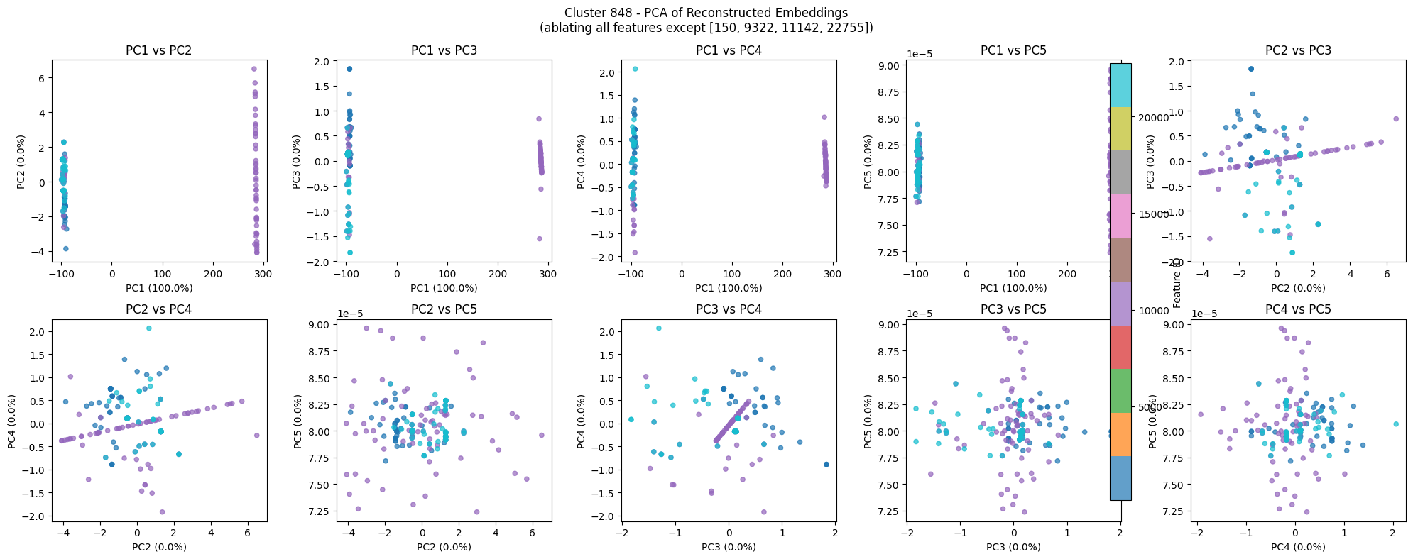
Figure 8:A few PCA components of the reconstruction point cloud for cluster 848. Note that the persistence diagram below is not computed on just the 2-dimensional projection.
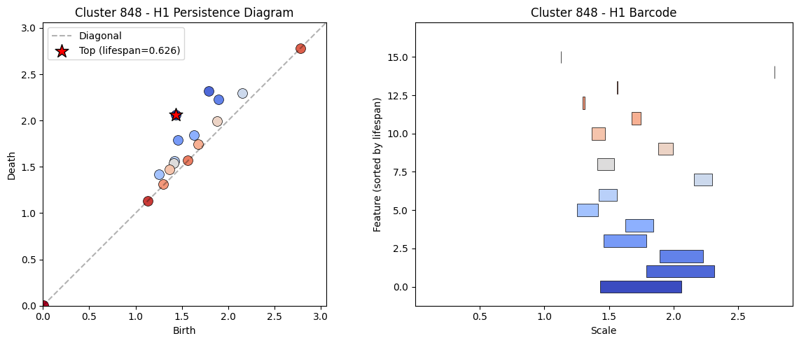
Figure 9:Persistence diagram (and equivalently barcode) for cluster 848.
The reconstructions are peculiar with a linear divider in the center of many of the plots, but with minor cycles forming around this linear component. The top activating tokens are also interesting.
Cluster 848 - Top Activating Features
Feature 150 - Top 10 tokens:
578- “578 F.2d”Warning- “Warning: Free hotel WiFi”999- “999 A.2d”999- “999 F.2d”663- “663 F.2d”985- “985 F.2d”District- “District Madhubani”2018- “2018 Grambling State Tigers”987- “987 A.2d”CRE- “CREATE TABLE mr”
Feature 9322 - Top 10 tokens:
att- “attached”et- “et v(p)”forth- “forthcoming in Noû”org- “org.springframework.”MAX- “MAXON NAB Works”WHO- “WHO Optim”MR- “MR imaging of post-”DE- “DEAL:0::”E- “Eucereon setosa”E- “Ein Mäd”
Feature 11142 - Top 10 tokens:
,- “On Friday, the 16-year”,- “ron Field Saturday, December 9 7”,- “Sent: Thursday, August 23, 2001”,- “will gather on Sunday, February 16 from 1”,- “Sent: Tuesday, April 03, 2001”,- “this Wednesday, August 2.”,- “4PM on Tuesday, October 23 or”,- “Sent: Monday, May 07, 2001”,- “urs Forum Thursday, October 25, 2001”,- “! Friday, March 16th”
Feature 22755 - Top 10 tokens:
forth- “forthcoming in Noû”later- “later today, someone will”att- “attached”DEM- “DEMOCRACY AND”org- “org.springframework.”iss- “issuer:ca”ter- “ter 5:01 AM”version- “version https://git-”version- “version: 1 n”d- “ditto on the response”
While far from perfect, the features do have clearer meaning, e.g. 11142 is clearly punctuation in the context of dates, while 150 is numbers in legal citation format. Upon prompting Claude in the same way as before, we obtain Formulaic text positions - 6.
The other plots and diagrams can be found in the top_persistence_spectral.ipynb notebook in the repository.
4.2.2Graph based clustering
Table 2:Significant (graph) Clusters (p < 0.05). Table depicts the 5 clusters with highest diameter and ratio scores respectively as well as the clusters containing temporal concepts (whose p-values are under 0.05) such as days of the week, months of the year, seasons, or times in the top activating tokens (or their context). Significance: * p<0.05, ** p<0.01
| Cluster | Type | Diam. Score | Diam. p-val | Ratio Score | Ratio p-val | ||
|---|---|---|---|---|---|---|---|
| 12873 | Top 5 Diam | 0.1197 | 0.0050 | ** | 1.3458 | 0.0547 | |
| 3016 | Top 5 Diam | 0.1153 | 0.0050 | ** | 1.5412 | 0.0149 | * |
| 6329 | Top 5 Diam | 0.1122 | 0.0050 | ** | 1.3744 | 0.0398 | * |
| 6533 | Top 5 Diam | 0.1095 | 0.0050 | ** | 1.5352 | 0.0149 | * |
| 2737 | Top 5 Diam | 0.1008 | 0.0050 | ** | 1.4958 | 0.0149 | * |
| 6414 | Temporal | 0.0484 | 0.0398 | * | 1.3813 | 0.0348 | * |
| 98 | Temporal | 0.0381 | 0.0498 | * | 1.3507 | 0.0498 | * |
| 2905 | Temporal | 0.0355 | 0.0647 | 1.3917 | 0.0299 | * | |
| 8138 | Temporal | 0.0308 | 0.0896 | 1.3775 | 0.0398 | * | |
| 10952 | Top 5 Ratio | 0.0172 | 0.1692 | 2.1289 | 0.0050 | ** | |
| 8594 | Top 5 Ratio | 0.0061 | 0.2587 | 1.9730 | 0.0100 | ** | |
| 245 | Temporal | 0.0030 | 0.2786 | 1.4248 | 0.0249 | * | |
| 8190 | Top 5 Ratio | 0.0000 | 0.2985 | 2.0000 | 0.0050 | ** | |
| 14210 | Top 5 Ratio | 0.0000 | 0.3085 | 2.0000 | 0.0050 | ** | |
| 2673 | Top 5 Ratio | 0.0000 | 0.3085 | 2.0000 | 0.0050 | ** |
The plots and diagrams here tell a similar story and can be found in top_persistence_graph.ipynb notebook in the repository.
- Maggs, K., Youssef, M., Pulver, C., Isma, J., Nguyên, T. J., Karthaus, W., Hess, K., & Dotto, G. P. (2025). CocycleHunter: cohomology-based circular gene set enrichment and genetic phase estimation in single-cell RNA-seq data. bioRxiv. 10.1101/2025.01.09.632214
- Engels, J., Michaud, E. J., Liao, I., Gurnee, W., & Tegmark, M. (2024). Not All Language Model Features Are One-Dimensionally Linear. arXiv. 10.48550/ARXIV.2405.14860
- Modell, A., Rubin-Delanchy, P., & Whiteley, N. (2025). The Origins of Representation Manifolds in Large Language Models. arXiv. 10.48550/ARXIV.2505.18235
- Carlsson, G., & Vejdemo-Johansson, M. (2021). Topological Data Analysis with Applications. Cambridge University Press. 10.1017/9781108975704
- Carlsson, G. (2009). Topology and data. Bulletin of the American Mathematical Society, 46(2), 255–308. 10.1090/S0273-0979-09-01249-X
- Edelsbrunner, H., & Morozov, D. (2013). Persistent Homology: Theory and Practice. In R. Latała, A. Ruciński, P. Strzelecki, J. Świątkowski, D. Wrzosek, & P. Zakrzewski (Eds.), European Congress of Mathematics Kraków, 2 – 7 July, 2012 (pp. 31–50). European Mathematical Society Publishing House. 10.4171/120-1/3
- Oudot, S. Y. (2015). Persistence theory: from quiver representations to data analysis. American Mathematical Society.
- Hatcher, A. (2002). Algebraic topology. Cambridge University Press.
- Editorial Board, G. (n.d.). Gudhi (3.7.1) [Computer software]. Inria. https://gudhi.inria.fr
- Bloom, J., Tigges, C., Duong, A., & Chanin, D. (2024). SAELens. https://github.com/decoderesearch/SAELens
- Templeton, A., Conerly, T., Marcus, J., Lindsey, J., Bricken, T., Chen, B., Pearce, A., Citro, C., Ameisen, E., Jones, A., Cunningham, H., Turner, N. L., McDougall, C., MacDiarmid, M., Freeman, C. D., Sumers, T. R., Rees, E., Batson, J., Jermyn, A., … Henighan, T. (2024). Scaling Monosemanticity: Extracting Interpretable Features from Claude 3 Sonnet. Transformer Circuits Thread. https://transformer-circuits.pub/2024/scaling-monosemanticity/index.html
- Simon, E., & Zou, J. (2025). InterPLM: discovering interpretable features in protein language models via sparse autoencoders. Nature Methods, 22(10), 2107–2117. 10.1038/s41592-025-02836-7
- Nanda, N., & Bloom, J. (2022). TransformerLens. https://github.com/TransformerLensOrg/TransformerLens