An Introduction to Mechanistic Interpretability of Neural Networks
Last week, we saw that transformer models (such as LLMs) are relatively simple architectures primarily built on simple linear algebra. Despite their simple mathematical building blocks, when scaled up (large amount of data, training for long periods of time, and increasing the number of layers) these models produce impressive results on a large range of tasks. Although scaling up in this manner delivers impressive results, they also exhibit a wide range of harmful behaviors such as hallucination (Ji et al. (2023)) or harmful content among others. Moreover, the models perform in unpredictable manner making deployment in sensitive domains such as medicine or law where decisions can significantly impact human lives challenging.
Mechanistic interpretability (MI) attempts to address these issues by reverse engineering transformer models by understanding small pieces of a model and how they interact with each other. By doing so, we hope to understand how these models represent features of interest and the internal computations by which they produce their outputs. If we were able to do this we could perhaps understand and prevent harmful behavior, e.g. by tuning weights appropriately.
Transformers (a quick recap)
Last week, we saw that transformers are built from some very simple mathematics - primarily linear algebra. The following section primarily follows Elhage et al. (2021), which is an excellent reference for the mathematics of a transformer with many pretty pictures. Recall that given a token, a transformer first embeds this token, passes this embedding through a series of residual blocks, followed by a finally unembedding layer that yields a probability distribution on the following token. Each residual block consists of an attention layer and a multilayer perceptron (MLP).
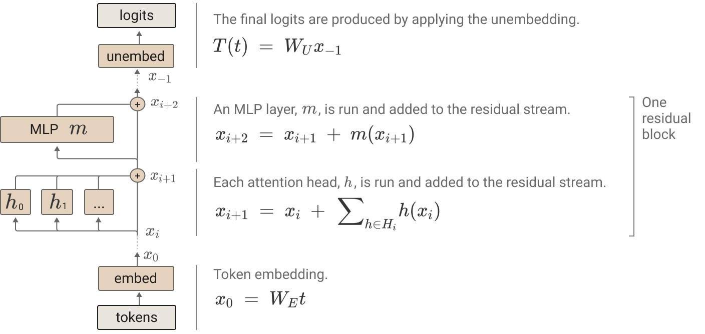
Figure 1:A transfomer architecture (Elhage et al. (2021)).
Rather than overwriting the results from previous layers, each layer of the residual block “reads” its input from the residual stream (by performing a linear projection), and then “writes” its result to the residual stream by adding a linear projection back in. Note that each attention layer consists of multiple heads which each act independently (adding their results to the residual stream). The residual stream is simply the sum of the output of the previous layers and the original embedding and should be thought of as a communication channel between layers.
Note that the residual stream has a very simply linear, additive structure - each layer performs an arbitrary linear transformation to “read in” information from the residual stream at the start, 4 and performs another arbitrary linear transformation before adding to “write” its output back into the residual stream. One basic consequence is that the residual stream doesn’t have a privileged basis; we could rotate it by rotating all the matrices interacting with it, without changing model behavior.
Features as the basic unit of neural networks
As stated above MI seeks to break up models into components, understand how these components work, and how they fit together. The first question we need to address therefore is: what is the fundamental/basic unit of a neural network? Intuitively, one might expect neurons to be this basic unit, and early research in mechanistic interpretability did indicate that this was true. For example, one of the first attempts in MI was Olah et al. (2020), where the authors examined InceptionV1 (Szegedy et al. (2015)) which was a CNN introduced by Google for image recognition. The authors find neurons that activate on specific features. For example, they find neurons that respond to curved lines and boundaries with a radius of around 60 pixels.
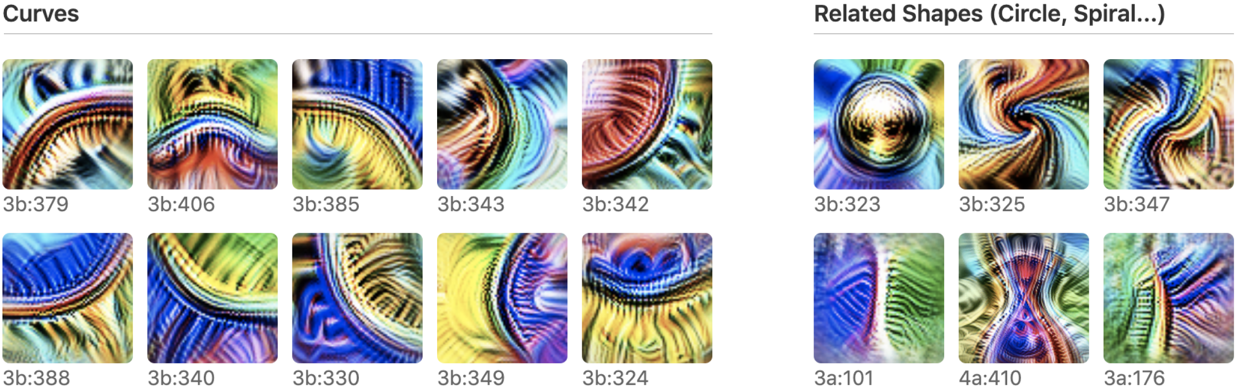
Figure 2:Examples of images on which curve detection neurons have high activation (Olah et al. (2020)).
There were other examples such as neurons that detected dog heads. These neurons are called monosemantic since they encode a single, well-defined concept. Often however, neurons appear to be polysemantic, i.e. a single neuron encodes multiple features.
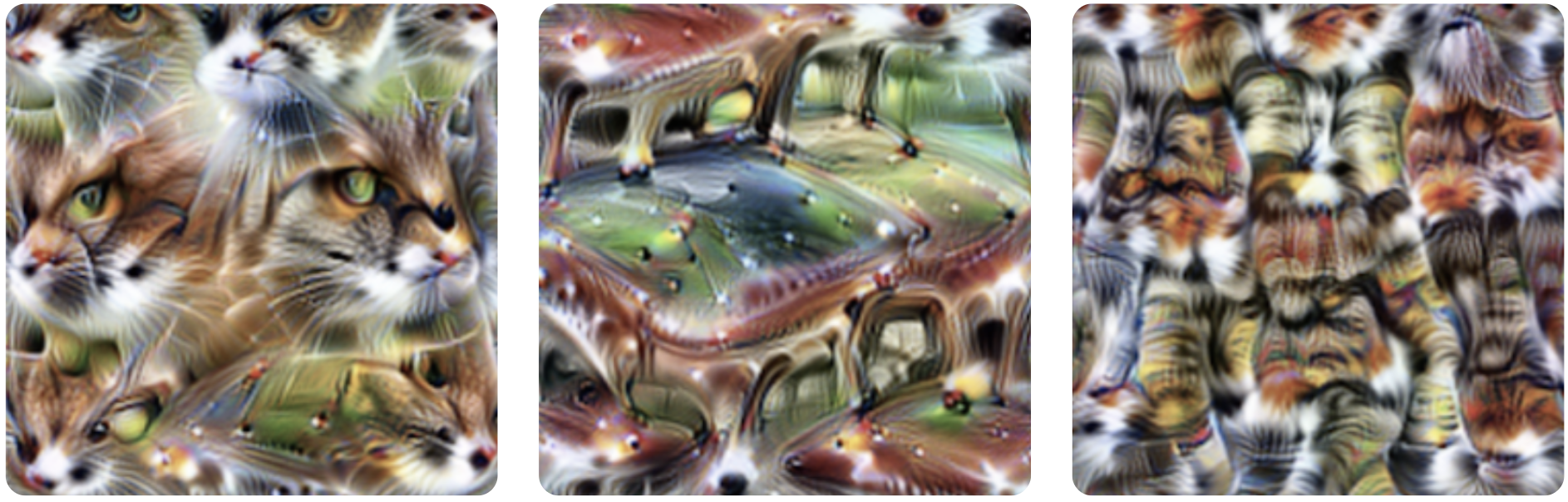
Figure 3:Examples of images which a single neuron responds strongly to (an example of polysemanticity) (Olah et al. (2020)).
The principle of superposition
It turns out that a large portion of neurons are polysemantic, even in simple models trained on data with few features. One explanation for this is the principle of superposition, which posits that when tasked with representing data with more independent “features” than it has neurons, it assigns each feature a linear combination of neurons. Intuitively, an LLM is attempting to encode trillions of “features” such as Python code, DNA, algebraic topology, sheaf theory, cellular biology etc with much fewer neurons. Essentially it is trying to encode a high dimensional vector space into a much lower dimensional one. Elhage et al. (2022) point to classical results that indicate that such a task is possible
Johnson-lindenstrauss Lemma: Suppose our model is attempting to represent data with underlying features but only has neurons at its disposal, such that . Faithfully approximating this data, amounts to finding low-distortion embeddings of into . The lemma guarantees that a linear map exists such that given orthogonal vectors the projections are quasi-orthogonal (i.e. ). In other words, it’s possible to have quasi-orthogonal vectors in .
Compressed sensing: The result allows us to project a high-dimensional vector onto a lower dimensional space, but how do we recover the original vector? In general, it is impossible to reconstruct the original vector from a low-dimensional projection, but results from the field of compressed sensing tell us that this is possible if the original vectors were sparse. This is the case for feature vectors, since each concept (e.g. text relating to enriched categories) only occurs relatively rarely in the overall dataset.
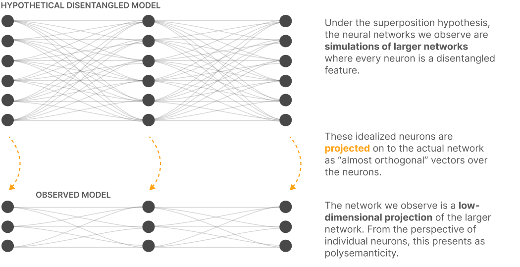
Figure 4:We can think of a neural network as approximating a larger sparse model (Elhage et al. (2022)).
In other words, we can think of a neural network as approximating some larger model by superposition. In the larger model (where we have as many neurons as features), neurons are monosemantic. The models we can build in practice use superposition to project these features onto polysemantic neurons.
The main takeaway here is that neurons exhibit polysemanticity and cannot be used as the fundamental unit of a neural network in the context of MI.
What is a feature?
Thus far, we’ve been talking about “features” without defining precisely what we mean by them. Intuitively these should be thought of as the intrinsic characteristics of the dataset the model is attempting to learn and that the model uses to represent the data. For example, InceptionV1 might have features such as curves, car doors, and dog faces among others that it uses to represent the dataset of images. An LLM might use features like category theory, politics, and Scotland among others as features that it believes represent the dataset of text. There are multiple approaches that one could take to define features such as (Elhage et al. (2022)):
(1) features as arbitrary functions of the input.
(2) features as interpretable properties i.e. things like curves or dog faces that are human interpretable.
(3) Features are neurons in sufficiently large models, i.e. the neurons in the large model that the observed model is attempting to approximate using superposition. Intituively, each neuron in the upper model depicted in Figure 4 forms a feature of the observed model downstairs.
Although (3) might seem circular, this interpretation yields features the model might actually learn (assuming the superposition hypothesis). This is not true of (1). Using (3) gives us a shot of extracting features the model cares about, while (2) restricts to concepts that we understand. Finally, as we will see below (3) is easy to operationalize.
Formally, this definition uses the superposition hypothesis to state the following. Consider a single block transformer model, i.e. a transformer with a single attention layer and a single MLP layer. Let denote the number of neurons in the MLP layer. Then the activation space of the model is (each of the neurons can take on a single real value). Each token yields a vector when fed through the MLP layer. The superposition hypothesis states that this activation vector is an approximation as below
where is the activation of feature and is a unit vector in activation space called the direction of feature . Note that there are pairwise quasi-orthogonal feature directions . The fact that features are sparse means that for a given , for most .
Using features to determine the mechanics of a model
Suppose that we can express MLP activations as a linear combination of feature diections as above. Bricken et al. (2023) put forward desirable characteristics of such a decomposition:
Interpretatable conditions for feature activation: We can find a collection of tokens that cause feature to activate, i.e. is high and we can describe this collection of tokens.
Interpretable downstream effects: Tuning (forcing it to be high or low) results in predictable and interpretable effects on the token as it passes through to subsequent layers.
The feature faithfully approximates the function of the MLP layer: The right hand side of (1) approximates the left hand side well (as measured by a loss function).
A feature decomposition satisfying these criteria would allow us to (Bricken et al. (2023)):
Determine the contribution of a feature to the layer’s output, and the next layer’s activations, on a specific example.
Monitor the network for the activation of a specific feature (see e.g. speculation about safety-relevant features).
Change the behavior of the network in predictable ways by changing the values of some features. In multilayer models this could look like predictably influencing one layer by changing the feature activations in an earlier layer.
Demonstrate that the network has learned certain properties of the data.
Demonstrate that the network is using a given property of the data in producing its output on a specific example.
Design inputs meant to activate a given feature and elicit certain outputs.
Sparse Autoencoders
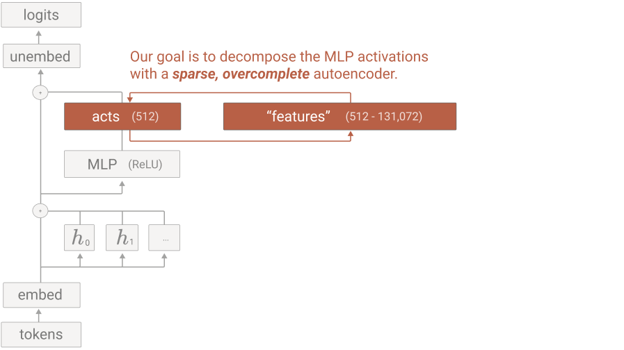
Figure 5:Decomposing MLP activations into features using a sparse, overcomplete autoencoder (Bricken et al. (2023)).
We learn feature directions and activations by training a sparse autoencoder (SAE). This is a simple neural network with two layers. The first layer is an encoder that takes in an activation vector and maps it to a higher-dimensional (say ) latent space using a linear transformation followed by a ReLU activation function. Denote by the learned encoder weights and by the biases. The second layer maps the latent space back down to -dimensions using a linear transformation. Denote by the learned decoder weights and by the biases. Applying the encoder and then the decoder to an activation vector yields
where
If and the features are sparse, we have an implementation of (1). The loss function we train the SAE on accomplishes exactly this
The first term ensures that the activation vectors are reconstructed faithfully while the second term ensures sparsity.
Experimental results
in Bricken et al. (2023), the authors train SAEs with increasingly higher latent dimensions on a simple single layer transformer. The results they obtain indicate that SAEs are capable of extracting interpretable features that
Activate with high specificity to a certain hypothesized context (by context we mean a description of the tokens that activate it like DNA features or Arabic script): whenever is high the token can be described by the hypothesized context.
Activate with high sensitivity to a certain hypothesized context: whenever a token is described by the context, is high.
Cause appropriate downstream behavior: Tuning (e.g. by setting to always be high regardless of the input token) and replacing by with results in outputs that reflect . Note that is obtained in the following way: for a given , run the model as is until we obtain the output of the MLP layer . Replace in the residual stream by running it through the SAE with the tuned version of and obtaining the reconstruction and let the following layers of the transformer proceed as is. A particularly impressive example of this is Golden Gate Claude (Templeton et al. (2024)), where the authors are able to scale up the SAE machinery developed in Bricken et al. (2023) to a full-blown version of Claude. They are able to pin point a feature that corresponds to the Golden Gate bridge and upon tuning that feature up (i.e. making high for all ), Claude outputs text related to the Golden Gate bridge regardless of the input.
Do not correspond to any single neuron.
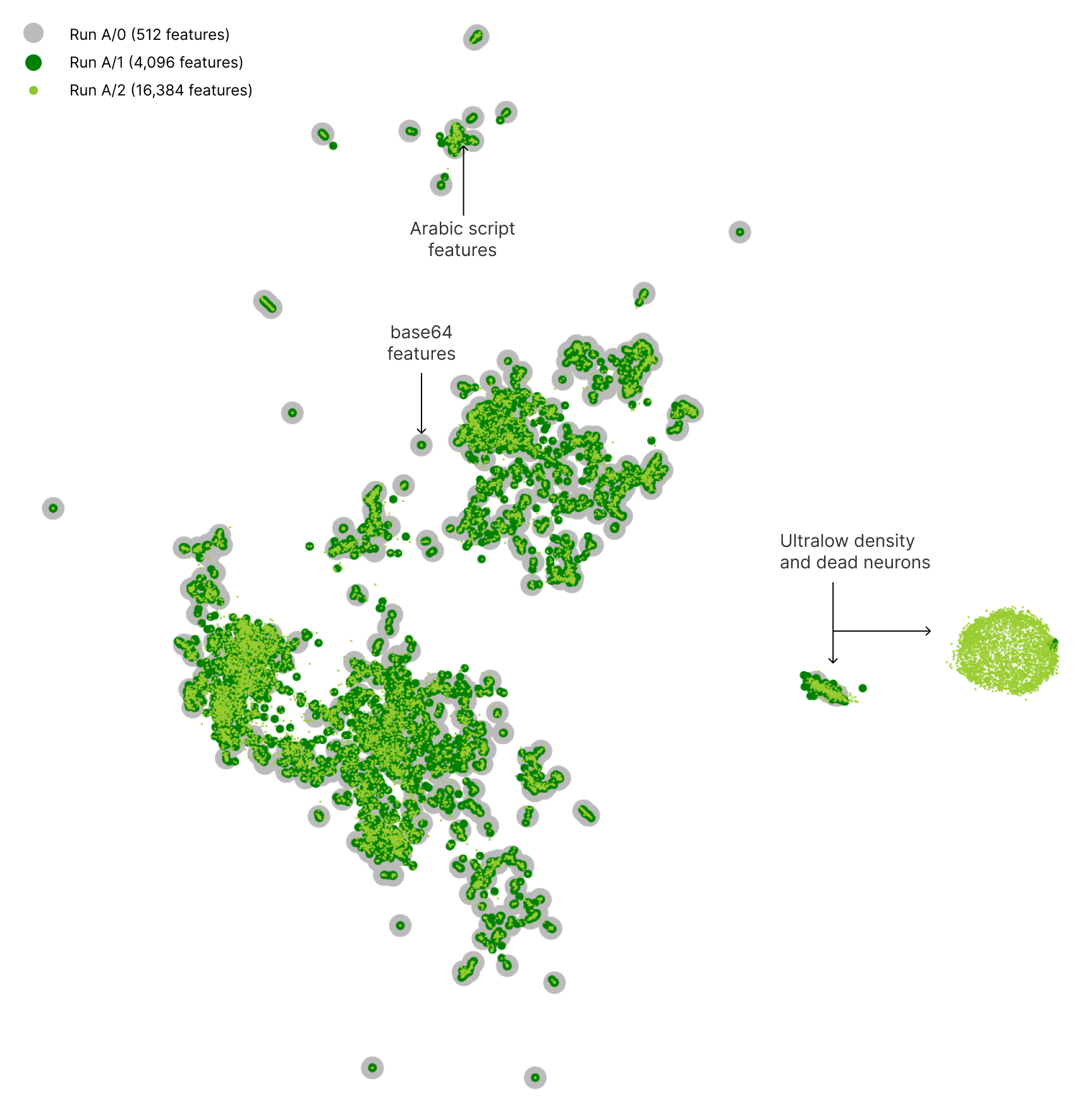
Figure 6:2D UMAP projection of the columns of the decoder matrix (feature directions) of sparse autoencoders with varying latent space dimensions (Bricken et al. (2023)).
I strongly recommend going through Bricken et al. (2023), as the visualizations of the features they find are very cool! The interactive dashboard lets you explore features, the tokens that activate them, the effects of ablating (tuning) features, and descriptions of features among other things. One particularly striking observation is that feature directions (the columns of the decoder matrix of the sparse autoencoder) appear to cluster as seen in Figure 6. The image shows feature directions of sparse autoencoders with different latent dimensions (the gray is a sparse autoencoder with 512 latent dimensions while the light green points are feature directions of an encoder with latent dimensions). Similar concepts such as those corresponding to Arabic script or base64 appear to cluster together. To me this is rather counterintuitive as I would have expected a more uniform distribution in order to minimize interference.
- Ji, Z., Lee, N., Frieske, R., Yu, T., Su, D., Xu, Y., Ishii, E., Bang, Y. J., Madotto, A., & Fung, P. (2023). Survey of Hallucination in Natural Language Generation. ACM Comput. Surv., 55(12). 10.1145/3571730
- Rauker, T., Ho, A., Casper, S., & Hadfield-Menell, D. (2023). Toward Transparent AI: A Survey on Interpreting the Inner Structures of Deep Neural Networks. 2023 IEEE Conference on Secure and Trustworthy Machine Learning (SaTML), 464–483. 10.1109/SaTML54575.2023.00039
- Elhage, N., Nanda, N., Olsson, C., Henighan, T., Joseph, N., Mann, B., Askell, A., Bai, Y., Chen, A., Conerly, T., DasSarma, N., Drain, D., Ganguli, D., Hatfield-Dodds, Z., Hernandez, D., Jones, A., Kernion, J., Lovitt, L., Ndousse, K., … Olah, C. (2021). A Mathematical Framework for Transformer Circuits. Transformer Circuits Thread.
- Olah, C., Cammarata, N., Schubert, L., Goh, G., Petrov, M., & Carter, S. (2020). Zoom In: An Introduction to Circuits. Distill, 5(3), 10.23915/distill.00024.001. 10.23915/distill.00024.001
- Szegedy, C., Liu, W., Jia, Y., Sermanet, P., Reed, S., Anguelov, D., Erhan, D., Vanhoucke, V., & Rabinovich, A. (2015). Going deeper with convolutions. 2015 IEEE Conference on Computer Vision and Pattern Recognition (CVPR), 1–9. 10.1109/CVPR.2015.7298594
- Elhage, N., Hume, T., Olsson, C., Schiefer, N., Henighan, T., Kravec, S., Hatfield-Dodds, Z., Lasenby, R., Drain, D., Chen, C., Grosse, R., McCandlish, S., Kaplan, J., Amodei, D., Wattenberg, M., & Olah, C. (2022). Toy Models of Superposition. Transformer Circuits Thread.
- Bricken, T., Templeton, A., Batson, J., Chen, B., Jermyn, A., Conerly, T., Turner, N., Anil, C., Denison, C., Askell, A., Lasenby, R., Wu, Y., Kravec, S., Schiefer, N., Maxwell, T., Joseph, N., Hatfield-Dodds, Z., Tamkin, A., Nguyen, K., … Olah, C. (2023). Towards Monosemanticity: Decomposing Language Models With Dictionary Learning. Transformer Circuits Thread.
- Templeton, A., Conerly, T., Marcus, J., Lindsey, J., Bricken, T., Chen, B., Pearce, A., Citro, C., Ameisen, E., Jones, A., Cunningham, H., Turner, N. L., McDougall, C., MacDiarmid, M., Freeman, C. D., Sumers, T. R., Rees, E., Batson, J., Jermyn, A., … Henighan, T. (2024). Scaling Monosemanticity: Extracting Interpretable Features from Claude 3 Sonnet. Transformer Circuits Thread. https://transformer-circuits.pub/2024/scaling-monosemanticity/index.html
- Modell, A., Rubin-Delanchy, P., & Whiteley, N. (2025). The Origins of Representation Manifolds in Large Language Models. arXiv. 10.48550/ARXIV.2505.18235